Learned Graph Structure for Learned Robot Dynamics

April 28, 2021

Learned Graph Structure for Walker2D and Cheetah

Intro

Learned dynamics models have been extensively applied in planning and control for a wide variety of robotics tasks. These models are useful because they allow us to model environment state transition dynamics simply from a dataset of interactions, instead of manually programming a first-principles simulator, which can be very expensive and may not accurately capture the true environment dynamics. Recently, there has been growing interest in parametrizing dynamics models as graphical models, as this class of models naturally capture the dependencies in the behavior of complex mechanical systems. The inductive biases that these graphical models provide have the potential to reduce model size and improve generalization performance over the standard multi-layer perceptron. However, most implementations have assumed that the graphical structure of the mechanical system is known a priori. While this may be a safe assumption for very simple systems, this assumption does not hold for complex systems with many links and actuators. Furthermore, it is possible that even for simple systems, a structure that captures all of the relationships may not be evident a priori. For example, for a legged robot, we could na ̈ıvely describe links as nodes, and add edges for every joint. However, we may find that due to the nature of the gaits that we could also add edges between opposite legs, due to the dependencies imposed by the gait. Therefore, we aim to address the challenge of learning the graph structure of a given dynamical system for the inference of the system’s dynamics

Model Architecture

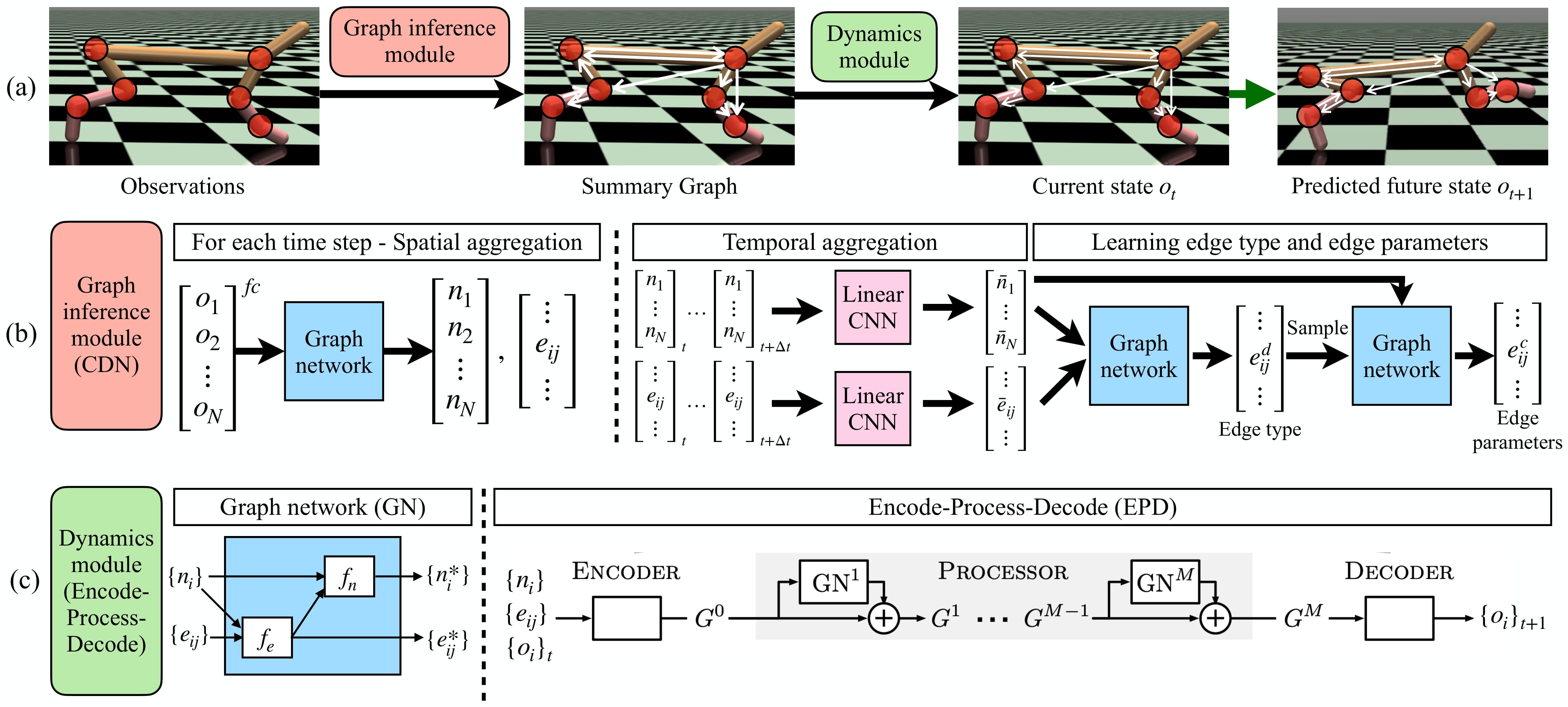
The above picture shows our full architecture.

(a) Learning architecture: Using observed trajectories the causal summary graph is inferred using the Inference module. The dynamics of the system is simultaneously learned using the Dynamics module that operates on the identified graph.
(b) Inference module discovers the edge set and the associated parameters. First, we propagate information spatially at each time step using a graph network which inputs a fully connected graph over all nodes. The output node and edge embeddings are then aggregated temporally and fed into a 1D-CNN to output temporal aggregations which are again be passed though another graph network that predicts a discrete distribution over edge types. Sampling from this distribution using the Gumbel-Softmax technique and passing through another graph network then gives the continuous edge parameters. The edge types and edge parameters together constitute the causal graph.
(c) Dynamics module: The left half of this subplot shows the graph network building block which acts as a single message passing step. The encoder encodes the node and edge parameters and observations and feeds them to the processor which acts like a sequence of message passing steps with skip connections. The output is then passed through the decoder which predicts the next state.

Qualitative Results

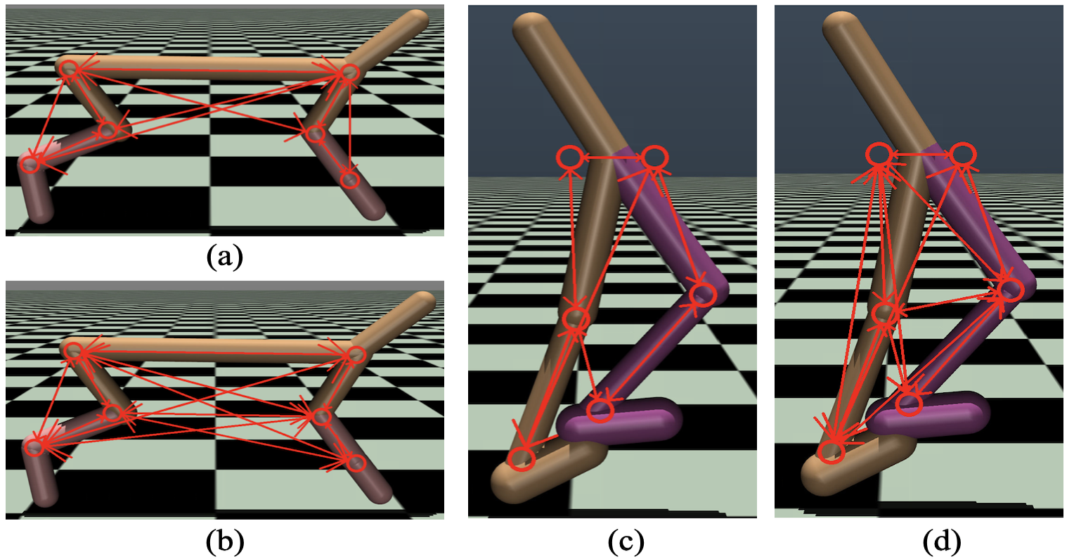
The figure at the top of the page visualizes the learned edges (directed arrows) and a priori known nodes (circles) annotated on top of the simulation models.

(a) shows the output of our CDN-EPD model, which resembles an almost fully-connected graph. This shows that the model was not able to identify the most meaningful edges, explaining the poor prediction performance.
(b) shows the output of CDN-GN, which is more sparse with dense connections only between nodes on the same leg. This matches our intuition since joints that are physically connected or spatially nearby should have edges. Only a few edges are learned across the two legs, and this possibly represents the relationship between the two legs in a gallop or walking motion since the legs follow a cyclic motion pattern. This shows the promise of learning a graph to discover useful relationships rather than assuming fixed priors.
(c) and (d) show similar trends.

Quantitative Results

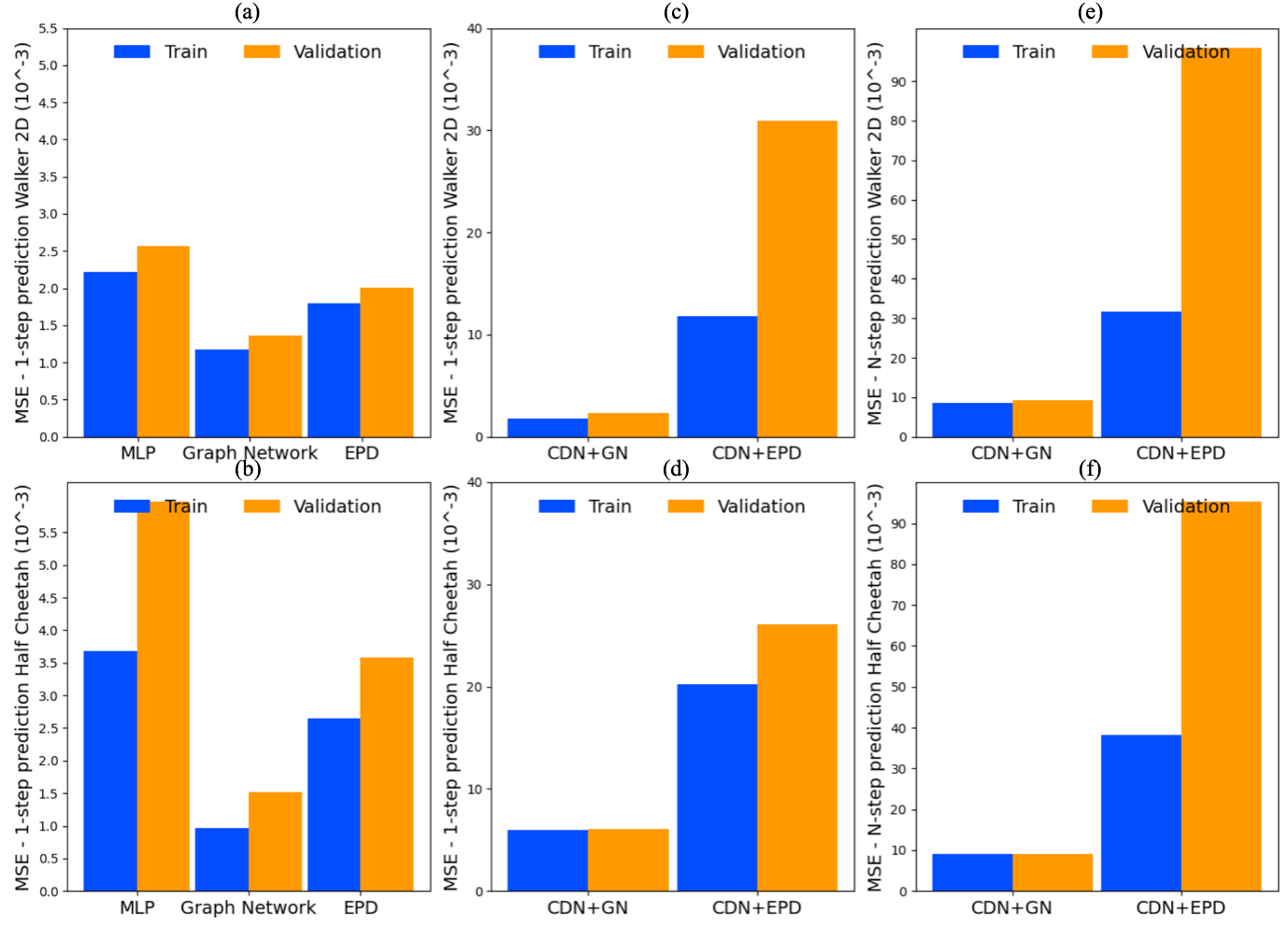
In all experiments, we find that the performance of the EPD dynamics model is worse than that of the GN model. We hypothesize that this is a result of the additional hyperparameters that the EPD model introduced, which may not be tuned correctly. Specifically, we believe that varying the number of message passing steps EPD performs (currently performing 10), may have a significant influence on performance, as GN per- forms better with a single step. Additionally, the added complexity of the model may be causing the joint optimization between the graph inference network and the dynamics prediction to settle into a local minimum, resulting in the mostly fully-connected graphs we see in the top figures (c) and (d). A potential fix for avoiding local optima could be pretraining the dynamics model based on a heuristic a priori graph.

Alvin Shek

Robotics Masters Student @ CMU

Robotics, Computer Vision, Deep Learning, Reinforcement Learning.